Please read Part 1 of the tutorial before proceeding with this one

Introduction

We mentioned some ideas in the last part by which we can abstract some parts of the Attention mechanism and make it more generalizable. In this part, we will go over a series of abstractions step by step and also understand the math with examples to build attention as a tool that we can use to attend over any set of input features when we are generating a sequence of outputs.

The flow for this part is hugely inspired by the Deep Learning for Computer Vision Course [10] at the University of Michigan and I have heavily borrowed from the explanations, so do watch that lecture series (after reading this post of course)!

Quick recap

In Part 1 we had built a complete attention-based system that could process input features in the form of a sequence of input tokens and apply attention using a feed-forward neural network. Also, remember that the purpose of the attention layer is to produce a vector that effectively summarizes the input features depending on the output we are generating. We had seen this applied to the encoder-decoder architecture.

Abstraction 1: The input features

The input features do not need to be sequential, like the output from an encoder RNN like we saw in the previous post. We can have a set of input features and choose to attend over these features.

Let's apply this abstraction to a new task of image captioning. The main motive here is to show you how we can apply attention to an arbitrary set of input features.

The task of image captioning is to take an image as input and produce a caption for the image.

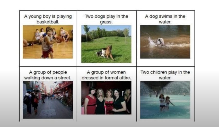Fig 1: Image captioning examples

We will still be using an encoder-decoder based architecture for this problem, but this time the encoder will be a Convolutional Neural Network (CNN). Typically a stack of CNN and fully-connected layers are used which take in the image pixels and compute a feature set - a feature set output from a CNN network is a grid of features in the form of a feature map.

If you are aware of how CNNs work, then this should be familiar to you. Otherwise, simply imagine that the output of the CNN is a grid of numerical values that encode spatial features about the image. At a very high level, you can imagine that the CNN has detected specific objects in the image as shown in the diagram below and the numerical values in the highlighted locations correspond to those objects.

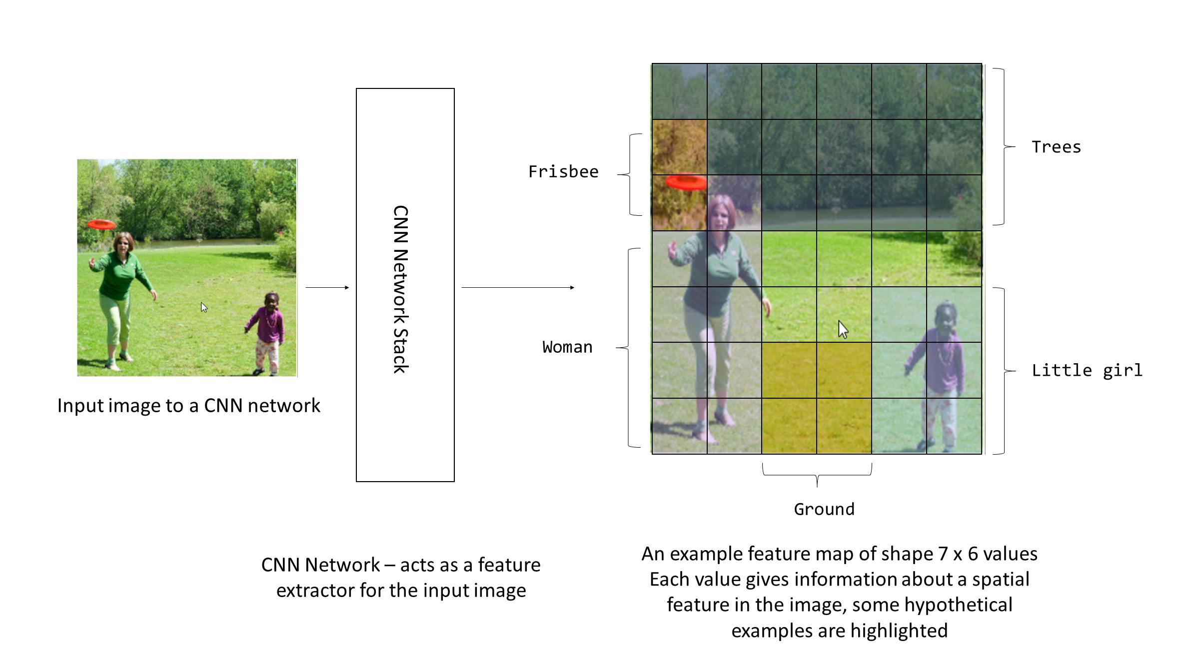Fig 2: Hypothetical feature set extracted from CNN

So the output of this CNN network is basically a grid of feature values that encode some useful information about the image that helps the network generate the corresponding captions. Here I have assumed that these features correspond to the objects in the image.

Notice how this is very similar to the previous task in which encoder RNN detected a set of features about an input sentence. Here we have an encoder CNN detect a grid of features about an input image.

We had a set of attention weights for the set of input features, similarly here we will build a grid of attention weights for the grid of input features.

Animation 1: Attention mechanism applied to the output from CNN (single time step shown)

Here we have shown for a single context vector c_t which will be fed to the decoder. But the key here is that at each time step this context vector is calculated by attending over different locations of the image, so you can imagine that when the model needs to output the word "frisbee" we can the weights highlighted in Fig 2 around the frisbee will be high.

Abstraction 2: The Neural Network for computing attention - replace with a simple dot product

Equation 3: The attention weights are learned by a neural network

We have mentioned previously that the function f_att which computes the attention weights, taking as inputs the hidden state vector and the input features. This function is learned by a feed-forward neural network.

What does this neural network do? It takes in the previous hidden state and the input features and computes a set of weights that determine how closely the input features interact with the previous hidden state in order to predict the output - so a loose assumption we can make here is that this NN is like a similarity function between the previous hidden state and the input features - I know that this seems like an oversimplification but for now, just understand that essentially what the NN is doing is figuring out how closely aligned (similar) each input feature is to the hidden state to predict the output.

We have already seen in Part 1 how a dot product is an excellent measure of similarity between 2 vectors - so let's try and replace this NN with a simple dot product - this will help reduce computation significantly as we do not need to train the NN to predict each attention weight!

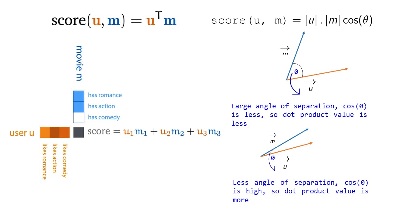Fig 3: The dot product as a similarity metric

The following sections will be a bit math-heavy but we will walk through an example time step to show how exactly these calculations are made. I would strongly suggest working through the math yourself (especially pay close "attention" to the matrix and vector shapes)!

Some notation conventions used:

Step 1: Initializing the variables

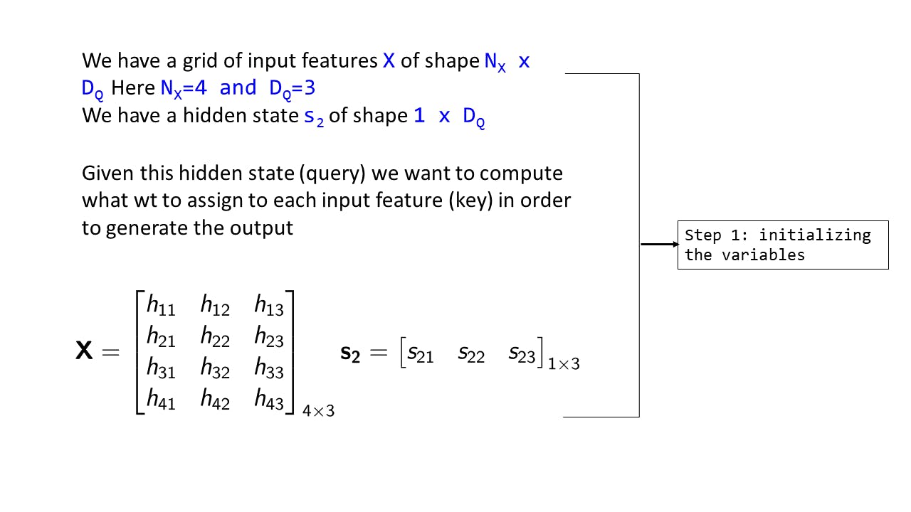Fig 4: Step 1 : Initializing the variables

• Assume we are currently on time step t=2, so we have the hidden state s₂. Each element of s₂, s_xy signifies : At time step x, the yth dimension of hidden state/query vector

• Assume that the hidden state has a dimensionality of 3 (D_Q)

• We assume we have the input features in a grid of shape N_X×D_Q (Here 4x3). This means that we have 4 input features, each of dimensionality 3. h_xy signifies the yth dimension of xth input feature

• We want to find: for this hidden state s₂, what are the weights we should assign to the input features in order to predict the output. So the hidden state is like a query, which is to be applied over the keys, which are the input features.

The task here is to understand how the vector s₂ interacts with each input feature. In terms of query and keys, we are trying to understand that given a hidden state vector (query) how does it interact with each of the input features (keys) - this is the basic motivation for the QKV architecture which is used in Transformers [1]

Step 2: Computing the raw Attention weights

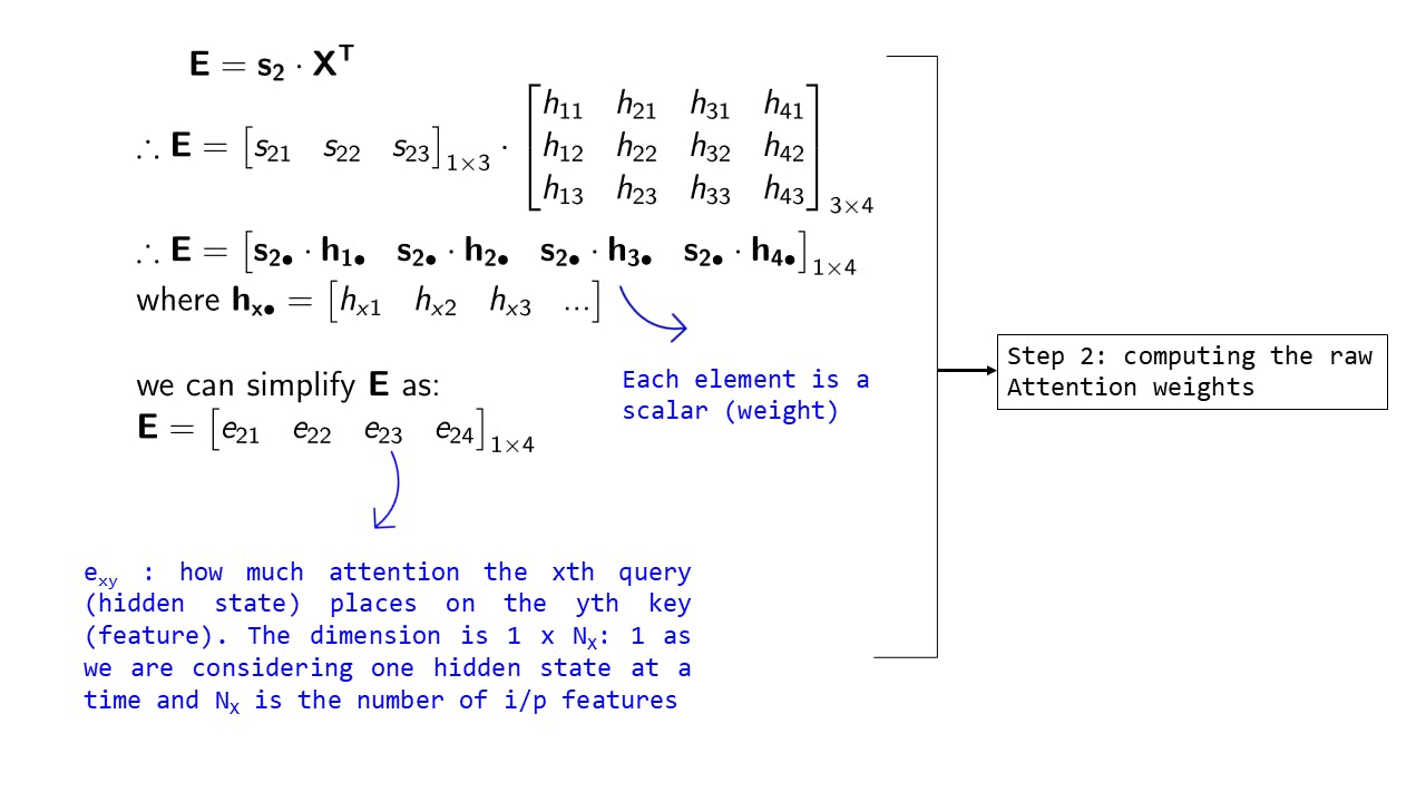Fig 5: Step 2 : Computing the raw Attention weights

• Previously as you can see in animation 1 we had computed each attention weight using the function f_att. Now as we are using the dot product, we can simply compute:

this allows us to get the set of attention weights in a single operation

• E is the set of attention weights over each input feature. the dimension of E is 1 x N_x - a weight for each input feature

• Also note that we have used a new notation a_x•. This is simply a cleaner way to write vectors. What it means is that keeping the first dimension of a fixed we expand along the second dimension (the dimension where the • is present). Just for clarity I could have avoided this notation, but if you look at explanations in this field where matrix-vector or matrix-matrix multiplications are used, then this notation is often used.

Step 3: Normalizing the raw Attention weights

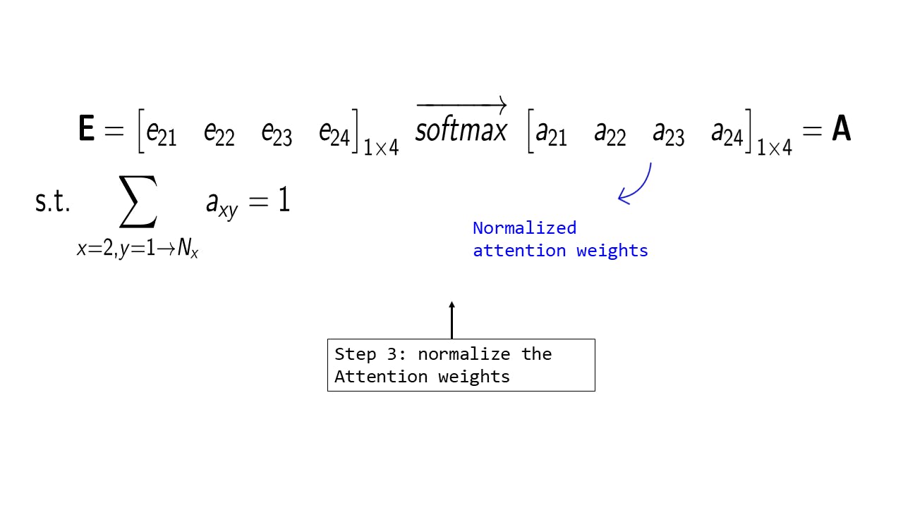Fig 6: Step 3 : Normalizing the raw Attention weights

This is a self-explanatory step in which we simply apply the SoftMax operation [6] to convert the raw attention weights to a probability distribution. Note that we now have a set of 4 weights that tells us that on a scale of 1-100 what percentage of attention we should provide to each input feature, given this current query vector - hopefully, you can see how interpretable and intuitive this is!

Step 4: Computing the output vector

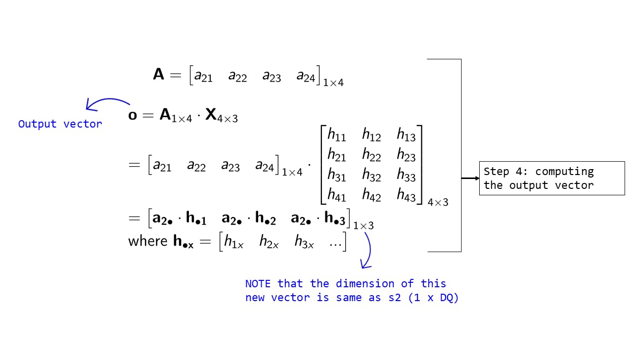Fig 7: Step 4 : Computing the output vector

• The output vector o is defined as o = A.X

• The shape of this vector is the same as the previous query vector - we can use this vector as the context vector to be fed into the decoder

To understand more concretely what this output vector looks like let's zoom into one of the terms:

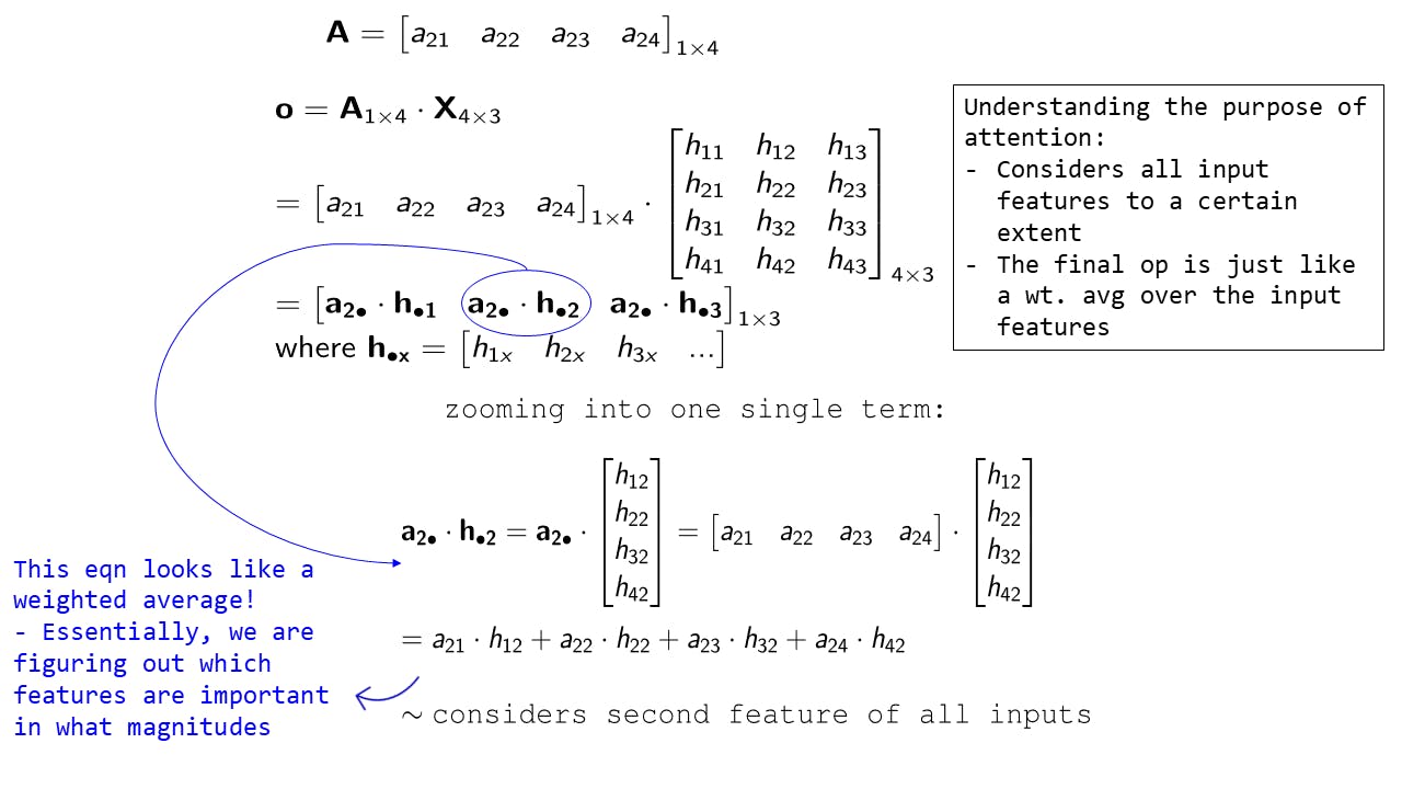Fig 8: Expanding one of the output terms

• Here we have picked the term a_2• . h_•2 and expanded it - as you can see it's simply a weighted average of each of the input features (considering the second dimension).

• Similarly a_2• . h_•1 would be a weighted average of each of the input features along the first dimension and a_2• . h_•3 will be the same for the 3rd dimension

• Thus we are considering each input feature to a certain extent and taking into account each dimension of the input feature. If you imagine for a traditional ML tabular dataset, each input feature is like an observation and each dimension is a feature.

Abstraction 3: Generalizing for multiple query vectors

We have abstracted the attention mechanism in a couple of ways so far:

1. It can work on any type of input features (keys)
2. We have replaced the neural network with the dot product between each key and the query vector to calculate the attention weights
3. But still the query vectors are fed into the attention mechanism one at a time, in the above example, we saw for the query vector s₂. We want to be able to input a matrix of query vectors and get the outputs out in a single time step.

The process remains largely the same as the previous one, the only difference is that we now input a set of query vectors in form of a matrix. Let's go over each step as before:

Step 1: Initializing the variables

Assume we have N_Q query vectors each of dimension D_Q. So we essentially have a Query matrix of shape N_Q × D_Q. Here N_Q = 2 and D_Q = 3. The input features matrix X is same as before.

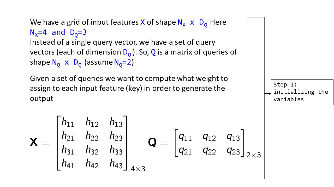Fig 9: Step 1 : Initializing the variables

Step 2: Computing the raw Attention weights

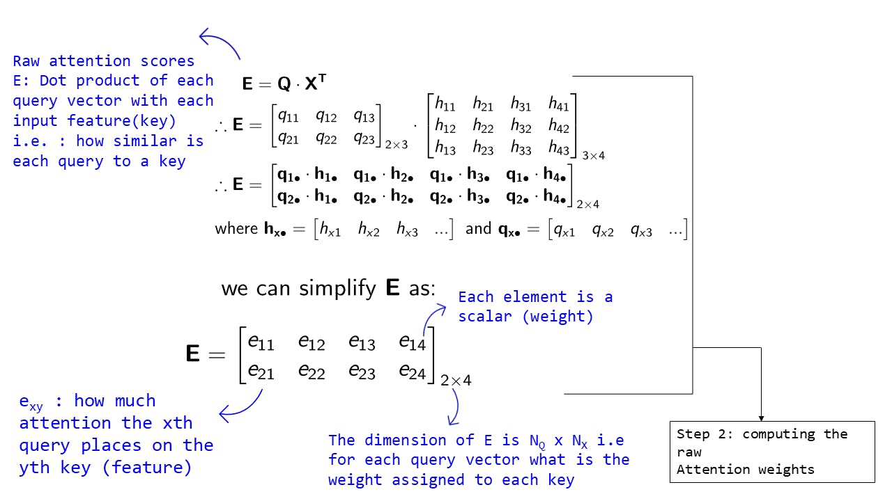Fig 10: Step 2 : Computing the raw Attention weights

• The equations are same as we saw before: This allows us to compute the attention weights for each query vector w.r.t each key in one single operation

• The interpretation of each raw attention weight e_xy is same as we saw before. The only difference is that E is a matrix instead of a vector as we are calculating for multiple query vectors. The dimension of E is N_QxN_X, i.e. for each query vector, what is the weight assigned to each key

Step 3: Normalizing the raw Attention weights

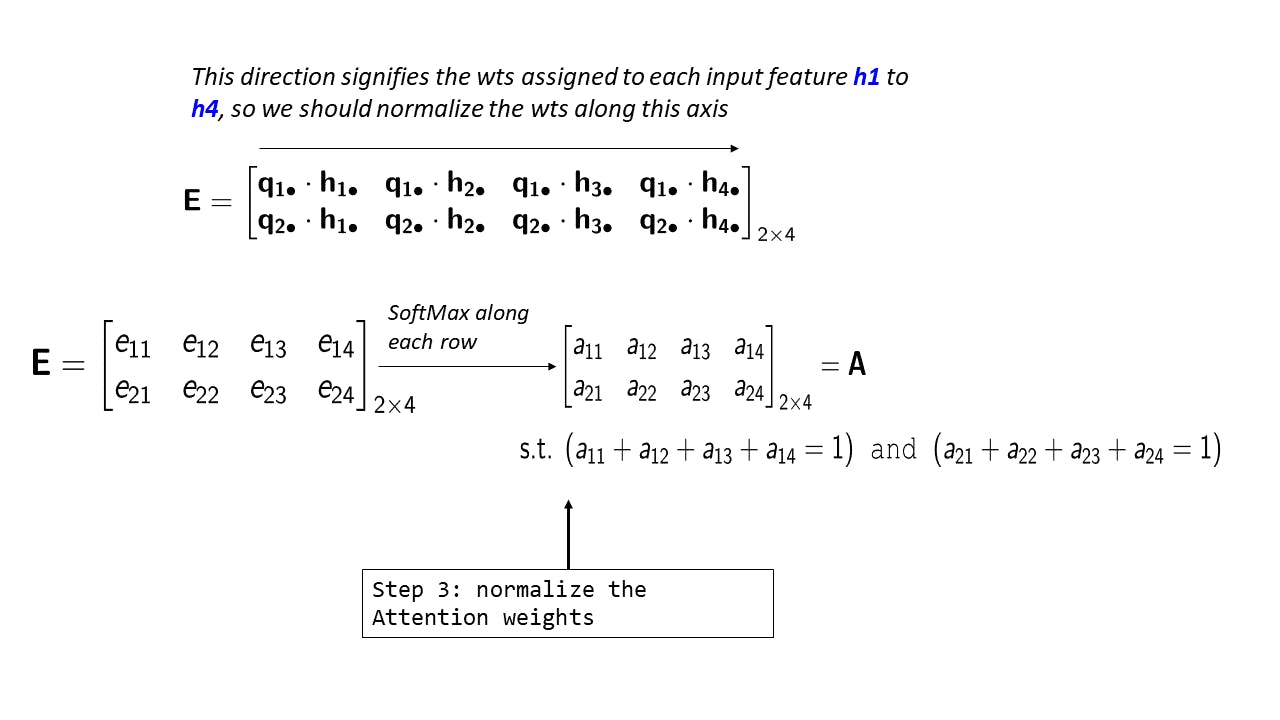Fig 11: Step 3 : Normalizing the raw Attention weights

E is the attention weight matrix. Each row of E contains N_X raw un-normalized weights, each weight corresponding to an input feature. There are N_Q such rows in E .

Now, for a particular query, each input feature gets assigned a weight and these weights need to be normalized, so we should apply the SoftMax operation on E along each row as shown in the above diagram.

Step 4: Computing the output matrix

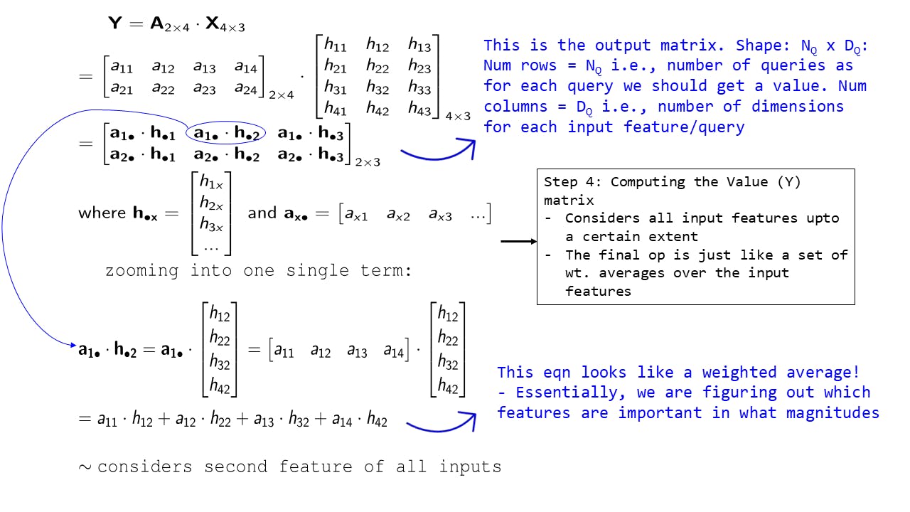Fig 12: Step 4: Computing the output matrix

In this step, we compute the output matrix. We will also call this the Value matrix.

The computation is the same as before and we get 2 rows as we had 2 queries. For each row, we have 3 dimensions (this is the number of dimensions in each query)

As before by zooming into one of the terms of the output we can see that each output value element is essentially nothing but a weighted average and that it considers a specific dimension of each of the 4 input features (in this case the second dimension)

Notice how the equations all remain the same, by simply stacking the query vectors as a matrix we can ensure that we can compute all values simultaneously.

Abstraction 4: Adding non-linearity and creating QKV Attention

Whenever we use attention mechanism we will have to define what our Queries, Keys, and Values are and how will they be constructed. At the end of this abstraction, you will have a great idea about how to build this and how this is used in Transformers. But let us first understand why this is even required.

First limitation: In the previous section, when we expanded out a term in the Value/Output matrix: a_1• . h_•2 and we saw that it's essentially a weighted average taking into account the 2nd dimension of each of the input features - while this is powerful and allows us to attend over the input features, its essentially a linear system. Also, we have replaced the function f_att which was learned by a neural network by dot products which are again linear. So we need some mechanism to incorporate non-linearity into attention.

Second limitation:: Also notice that we have used the input features matrix, i.e. the Keys in 2 different ways:

1. In Step 2 for calculating the raw attention weights as in:
2. In Step 4 for calculating the output/value matrix as in:

So basically the same matrix is used for 2 purposes - to determine which input features are important and also to return the actual output. These 2 are very different tasks - one for matching and one to actually return the matched output.

To emphasize this, imagine you are building a sequence predictor system and your system actually is a code-completion tool (something like OpenAI Codex ). So it takes as input an input text or comment and also the code written so far and should return the next few autocompleted lines of code.

Imagine you have asked the program to render a ball on the screen and it has written the code for you and displayed the ball. Now assume you give it the command - "Move it to the right by 100 px". If you have built attention into your system, you can expect this query to have assigned a strong weight to the input features or keys that correspond to the "ball" object - these might be the lines of code that have defined this object. But the value that we want to return is something like ball.x_position += 100, and not the features corresponding to the ball object. So the value that we want is an entirely different mapping of the input features than the keys. Essentially in this case:

Query: the docstring or comment specifying the command
Keys: i/p features that match that query
Value: code to execute the command

The solution is to simply use a transformation for getting the key matrix (K) and the value matrix (V) from the input features matrix (X). What transformation to use is simply learned by a neural network. So we learn the mapping from the input features to the Keys and Values.

Let's understand this process with the help of this animation:

Animation 2: Input features to Key Transformation

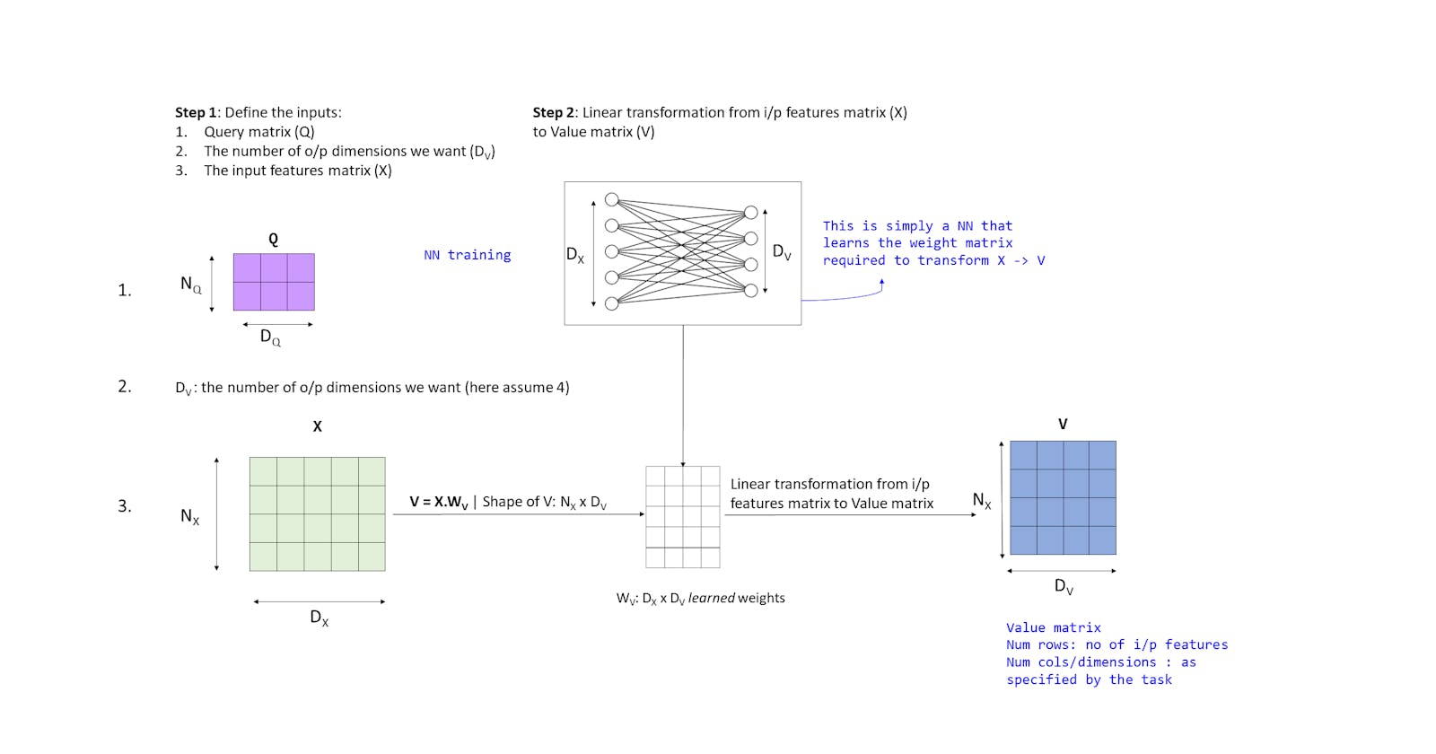
1. We define the following inputs:
   • Query matrix Q of shape N_Q×D_Q
   • D_V: the number of output dimensions we want
   • Input features matrix X of shape N_X×D_X
2. We build a neural network with D_X inputs and D_Q outputs which is trained to learn D_X×D_Q weights
3. We use these weights in form of a matrix W_K of shape D_X×D_Q to transform matrix X as: where the shape of K is N_X×D_Q - this is the same dimensionality as the input feature matrix considered in the previous examples.

We have obtained the Key matrix by learning a transformation from the input features. Since we are using a neural network to learn this, we can use a non-linear activation function like ReLU or sigmoid, so this brings an aspect of non-linearity in the system which solves our first limitation.

Similarly, we learn the Value matrix as shown below:

Animation 3: Input features to Value Transformation

1. The inputs are same as before
2. We build a neural network with D_X inputs and D_V outputs which is trained to learn D_X×D_V weights
3. We use these weights in form of a matrix W_V of shape D_X×D_V to transform matrix X as: where the shape of V is N_X×D_V

In this way we have successfully mapped out our input features into 2 transformations for Keys and Values. Now the rest of the operations remain the same - we just use the Key matrix K to compute the attention weights and use the Value matrix V to compute the output. Again the motivation is that, through these transformations, we can learn how to use the input features as Keys to match with the query vectors and as Values to return as the output.

Below we explain the process visually, these steps should be very familiar to you by now.

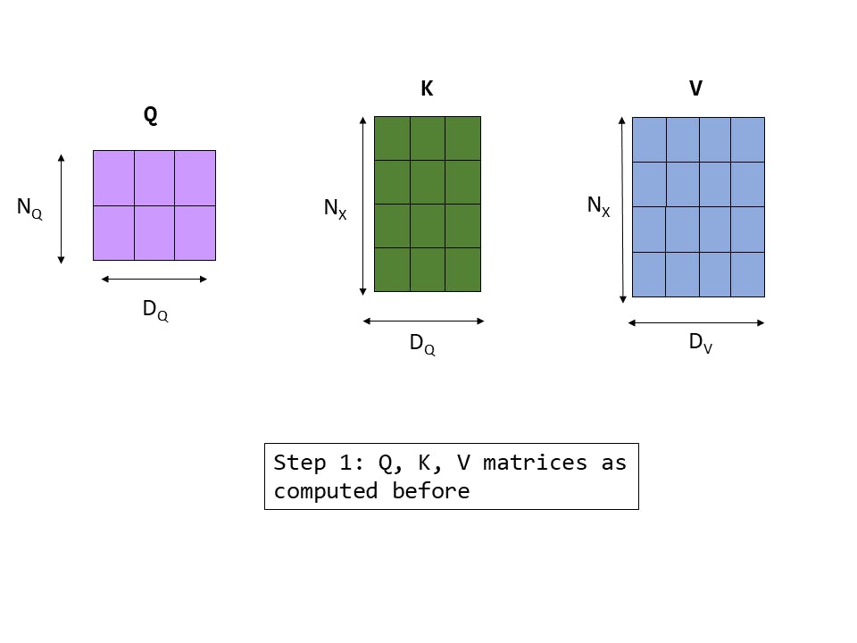Fig 12: Step 1 : QKV matrices computed as before

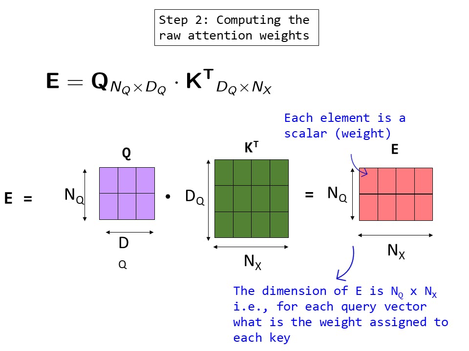Fig 13: Step 2: Computing the raw attention weights

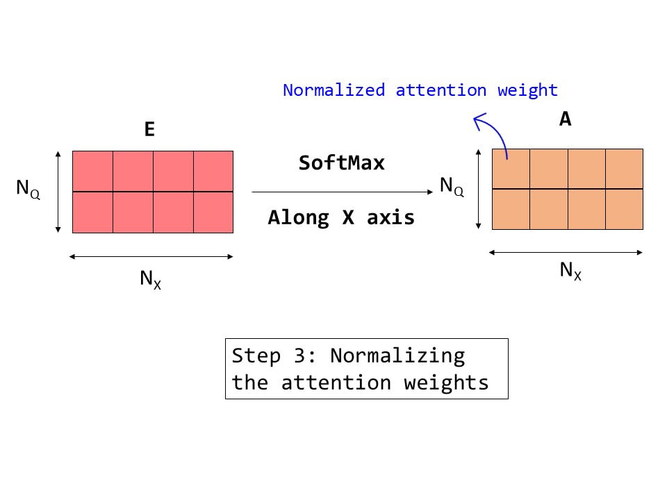Fig 14: Step 3: Normalizing the raw attention weights

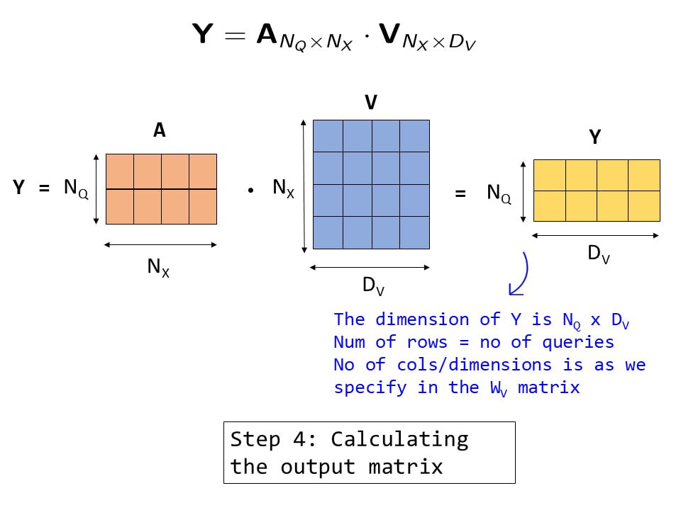Fig 15: Step 4: Computing the output matrix

The steps are exactly the same as we have done before, but we just use the newly built Keys and Value matrices to compute the attention weights and the final output matrix respectively.

This brings us to the end of this topic - we started from a form of attention that worked but was very specific and complex to a particular task as in Part 1 and built it up step by step in the form of these abstractions to generalize to the QKV form of attention that can be plugged into any transformer-based model [1].

---

Cite this article as:

@article{sen2021attention,
  title   = "Attention mechanism - An In-depth Analysis and Walkthrough - Part 2",
  author  = "Sen, Shaunak",
  journal = "https://shaunaksen.hashnode.dev",
  year    = "2021",
  url     = "https://shaunaksen.hashnode.dev/attention-mechanism-an-in-depth-analysis-and-walkthrough-part-2"
}

If you have any queries, spotted any errors, or simply want to leave feedback, do contact me at shaunak1105@gmail.com.

---

References

[1] Vaswani, Ashish, et al. “Attention Is All You Need.” ArXiv.Org, 12 June 2017, arxiv.org/abs/1706.03762.

[2] Sutskever, Ilya, et al. “Sequence to Sequence Learning with Neural Networks.” ArXiv.Org, 10 Sept. 2014, arxiv.org/abs/1409.3215.

[3] Mikolov, Tomas, et al. “Efficient Estimation of Word Representations in Vector Space.” ArXiv.Org, 7 Sept. 2013, arxiv.org/abs/1301.3781.

[4] Olah, Christopher. “Deep Learning, NLP, and Representations - Colah’s Blog.” Home - Colah’s Blog, 7 July 2014, colah.github.io/posts/2014-07-NLP-RNNs-Repr...

[5] Bloem, Peter. “Machine Learning @ VU | MLVU.” MLVU, mlvu.github.io. Accessed 22 Aug. 2021.

[6] Brownlee, Jason. “Softmax Activation Function with Python.” Machine Learning Mastery, 18 Oct. 2020, machinelearningmastery.com/softmax-activati...

[7] Weiss, Ron J., et al. “Sequence-to-Sequence Models Can Directly Translate Foreign Speech – Google Research.” Google Research, 2017, research.google/pubs/pub46151.

[8] Cho, Kyunghyun. “Introduction to Neural Machine Translation with GPUs (Part 2) | NVIDIA Developer Blog.” NVIDIA Developer Blog, 15 June 2015, developer.nvidia.com/blog/introduction-neur...

[9] Bahdanau, Dzmitry, et al. “Neural Machine Translation by Jointly Learning to Align and Translate.” ArXiv.Org, 1 Sept. 2014, arxiv.org/abs/1409.0473.

[10] Johnson, Justin. “EECS 498-007 / 598-005: Deep Learning for Computer Vision | Website for UMich EECS Course.” EECS 498-007 / 598-005: Deep Learning for Computer Vision, web.eecs.umich.edu/~justincj/teaching/eecs4... Accessed 22 Aug. 2021.