Introduction and pre-requisites

In this tutorial, you will learn about the Attention mechanism, a technique that is the backbone of the Transformers Neural Network architecture [1]. Transformers are state-of-the-art when it comes to natural language processing tasks like machine translation, code autocompletion, Named Entity Recognition, summarization, etc. It can even be used for computer vision tasks.

As you will see throughout this 2-part tutorial (link to Part 2), we will build attention from the ground-up - first, we will understand why it was needed, then build a working, but a specific version of the model at the end of this part. Then in the second part, we will work our way through a set of abstractions that help us generalize attention as a building block that we can insert in almost any neural network framework.

After completing the first part you will learn about:

1. The basic working of encoder-decoder architecture
2. The limitations of this architecture
3. The purpose of building an attention model and its intuition
4. Implementation and working of the attention model as a tool to improve the encoder-decoder architecture

Also before starting, I want to emphasize that while I have tried my best to provide context to each of the concepts covered here, there are quite a few pre-requisites to completing this tutorial:

1. Understand how neural networks work and how they are trained
2. Have a basic idea of what word embeddings are
3. A basic working of Recurrent Neural Networks and Convolution Neural Networks

Often, concepts in deep learning are not quite interpretable, but we will see this is not the case with the Attention mechanism and we will logically build towards the full architecture that is used in Transformers.

Tutorial Overview

1. A brief overview of the Encoder-Decoder architecture
   1. The input sequence
   2. Encoder stack of Neural Networks
   3. Hidden state vector/context vector
   4. Mapping of the hidden state → output word
      1. Dot product as a similarity measure
2. Limitations of this architecture
3. Building towards Attention
4. Next steps
5. References

A brief overview of the Encoder-Decoder architecture

In this section, we will be taking a high-level view of the popular encoder-decoder architecture [2] and get a basic idea of how it works. What has this got to do with Attention? - the limitations of this architecture inspired the attention mechanism and we will understand why these limitations occur and how to solve them.

The encoder-decoder architecture has 5 main parts that we want to talk about. These 5 parts are highlighted in the diagram below and we will understand them one by one.

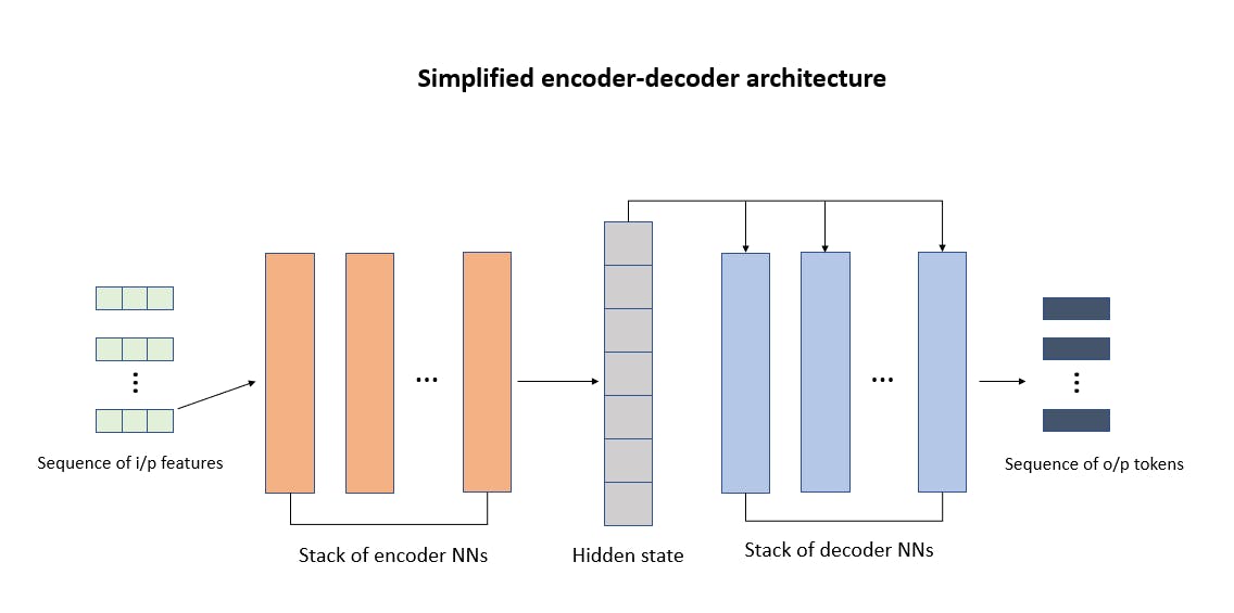Fig. 1: The basic seq -> seq architecture

1. The input sequence

Let us consider we are translating English to French. Let's assume that the sentence we want to translate is "Economic growth has slowed down in recent years." Then the input sequence is basically the tokens (individual words) of the sentence.

Now neural networks can't process raw text so we need to encode them in some numeric format. So each word should become a vector of numbers of a predefined dimension that we can input into the network. Why a vector and not a scalar - each word has multiple characteristics and vector allows for that information to be captured. Of course, we can use one-hot encoding for this purpose but a far better approach is to use word embeddings that can capture the similarities between the words. The word embeddings are typically learned through an algorithm like word2vec [3], which is a topic in itself, but you can imagine the output of this algorithm to be a vector for each word that encodes useful information about the word such that similar words, which are used together more often have similar embeddings and are thus, close together in vector space.

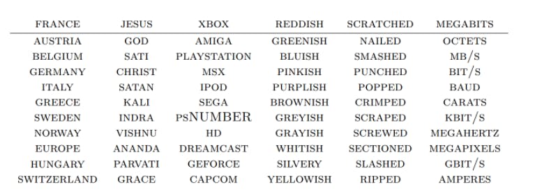Fig. 2: Which words are closest to an input word - [4]

To explain things very simply, we have a big embedding matrix with no of rows == no of words in vocabulary and no of cols/dimensions == no of dimensions we want each word to have - typically 64/128/512 (here we consider 4 for simplicity). We look up each word in the input sequence in this matrix and map it to a corresponding vector. This allows us to express each word as a vector and the way these vectors are defined is that words similar to each other are mapped closer to each other.

Animation 1 - Lookup each input word to its corresponding embedding

We can see in the animation above how each input token gets mapped to a corresponding vector. From now on, whenever you see me saying things like "the model receives a word as input", I mean that it takes in the learned vector corresponding to the word.

So the input sequence is basically a set of vector representations for each word.

2. Encoder stack of Neural Networks

A common misconception is that encoder-decoder architectures always use RNNs for encoding. But we can use any neural network which can take in a set of inputs and compute a set of features from it. And since all neural networks are feature extractors, we can use any neural network for this. We will see later in the post the use of CNN as the encoder to extract features from images. Here we will stick to RNNs as it will allow us to process sequential input.

For simplicity consider that the encoder comprises a single RNN block that processes each input token one by one. The working of this encoder RNN can be best understood with the help of an animation:

Animation 2 - Encoder animation

1. At each time step (t) the encoder RNN receives the current input x_t and the previous hidden state h_t-1. It then computes the next hidden state h_t (this hidden state will again be fed back to the network at time step t+1). In addition to the hidden step, the RNN also produces an output vector, which is not important for our use case
2. The initial hidden state h₀ is assumed to be all 0s
3. h₈ is the final hidden state

3. Hidden state vector/context vector

Thus the final op of this encoder block is h₈ of a specified dimension that basically summarizes all important information from the input sequence. This is because, to create h₈ we need to compute h₇, which in turn requires h₆ and so on. So the final hidden state vector can be referred to as the "context" vector as for a well-trained network this vector summarizes all useful information (features) from the input sentence that can be used by the decoder.

Notice how we loosely refer to this context vector as a set of features of the input text, so essentially the encoder network acts as a feature extractor for the input.

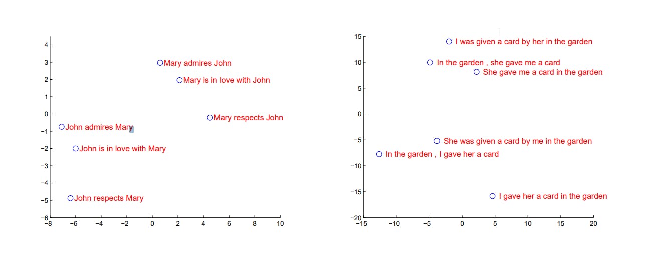Fig 3: Plot of the hidden state vectors of different sentences

In the above diagram, we plot the hidden state vectors for a number of input sentences. The authors in this paper [2] have used an LSTM network and used PCA to reduce the hidden state dimensions to 2 for plotting on the 2D coordinate system.

Notice how the hidden state seems to have efficiently encoded the input sentences as sentences of similar information are clustered together. Also, note that the input sentences are fairly short in these examples.

4. Decoder stack of Neural Networks

Now that we have a hidden state that has learned the important aspects (features) of the input sentence, we need a mechanism that can process this sequence of features and produce the outputs.

Again it is not necessary to use RNNs but since we are dealing with sequential data, for this task it makes sense to use a stack of RNNs as the decoder module. For simplicity, we consider that we have only one RNN as the decoder.

The RNN decoder, at each time step: t takes as inputs:

1. previous output word embedding op_t-1
2. previous hidden state s_t-1
3. the hidden state h₈ - the encoder output

Using these inputs the decoder basically computes: The next hidden state - s_t

The RNN decoder process can be summarized as:

Animation 3 - Decoder animation

There is a lot of things going on in this animation so let us go through it:

1. At the start we have the encoding process which takes in the word embeddings and computes a context vector h₈ as shown in Animation 2
2. At each time step the decoder computes the hidden state s_t using the equation :
3. Using this hidden state we map to an output word op_t which is the corresponding translated word in French - we will see what goes on in this "Mapping process to output" block soon.
4. Note that initially s₀ is set to a vector of 0s and op₀ is simply the embedding for the <START> token.

Let us understand what information each of the inputs provides to the decoder:

• previous output word embedding - given that the previous word generated was op_t-1 what should be the next word?
• previous hidden state - as each new hidden state s_t, is computed using s_t-1 which is calculated using s_t-2 and so on... So s_t captures information about all the outputs which have been generated so far, i.e.: given we have generated [op_1, op_2, ... op_k] what should be the next token to be generated
• h₈ - this gives information about the entire input sequence - this vector has summarized the input text and serves as a kind of "context" vector

So, to summarize at each step the decoder mainly tries to compute "given that I have generated the output: [op_1, op_2, ... op_k] and given that the previous word I generated was op_t-1 and given all the input features, what should be the next hidden state?"

5. Mapping of the hidden state → output word

We have so far seen how we use the decoder network to compute a vector s_t at each time step which is supposed to encode information about an output word - but how can we map this vector to an output word?

As we saw in Fig 1. we had a set of embedding vectors for each English word in form of a matrix from which we looked up the required input vectors. Similarly, we have the corresponding French word embeddings stored in a matrix. Once we get the hidden state s_t, we can compute the "similarity" between s_t and each French word embedding. We pick the word which gives the highest similarity score as op_t.

Dot product as a similarity measure

To explain this, let me borrow from the great course by Peter Bloem [5]. How it is explained there is: Imagine we have 2 vectors - for a movie m and for a user u.

Each dimension of these vectors is like a feature for the movie and user respectively and we can see that the movie has action in it and the user also likes action a lot.

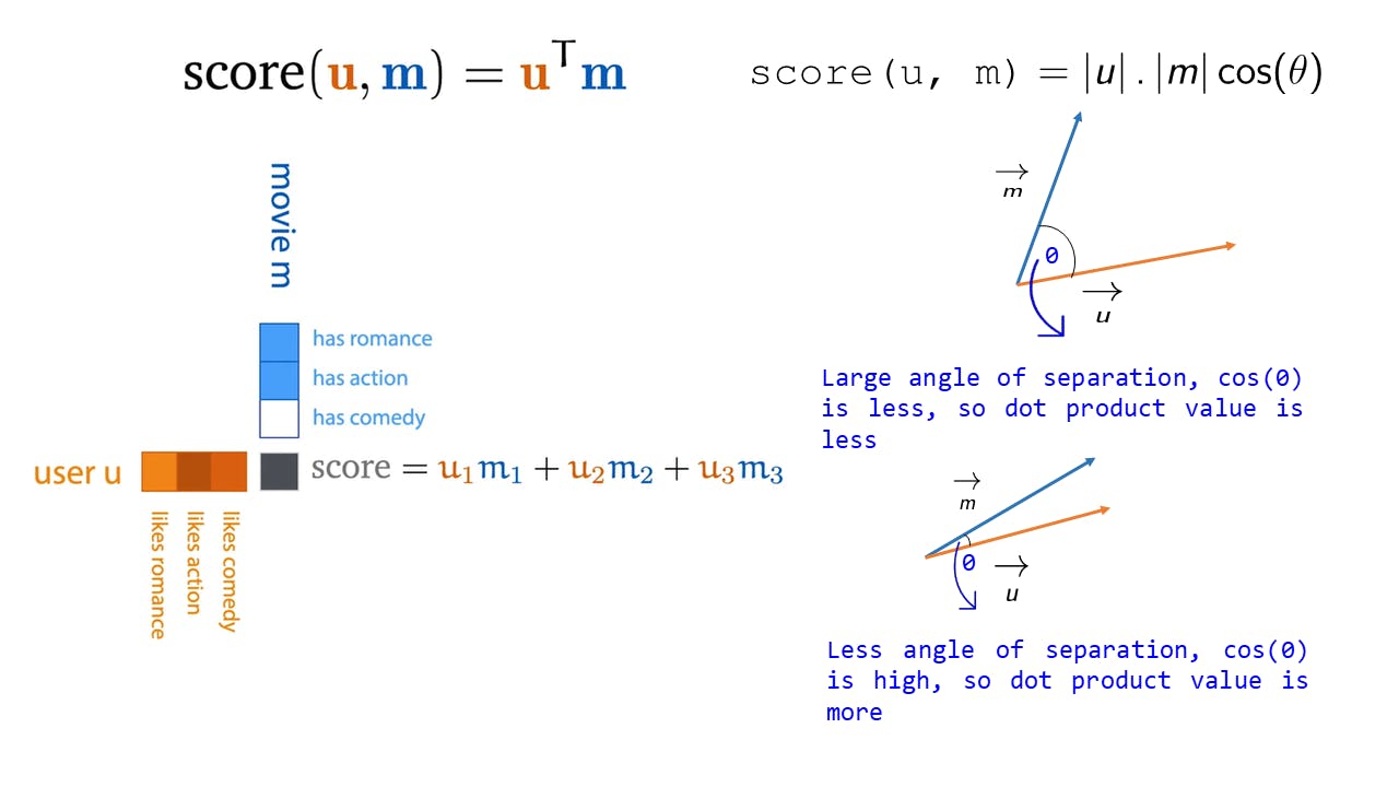Fig 4: Dot product explanation

The dot product between these two vectors gives us a score which is a scalar and its high in this case due to the fact that the user likes action and the movie has action - so the dot product returns a high value of score due to the large contribution of the term u_2.m_2 when the 2 vectors have similar features.

Similarly, we can imagine that if the user hates romance and the movie has romance then u_1 is a large negative, m_1 is a large positive and the score is low due to the negative contribution of the term u_1.m_1.

In terms of vector spaces, if we plot m and u, then if these vectors are closely aligned the dot product score is more, i.e. if the angle of separation θ is less, then cos(θ) will be more (for θ < 90 °: cos(θ) is monotonically decreasing function).

So, to conclude the dot product is a very intuitive and easy to compute metric for the similarity between 2 vectors.

Coming back to the original problem, we compute the dot product between s_t and each French word embedding - this gives us a set of similarity scores. These scores can range anywhere between (-∞, +∞) so we apply a softmax operation [6] to scale it to a range of [0,1] so that we can interpret these scores as probabilities. The intuitive reason for doing this is so that we can interpret the results for e.g.: "the translation of 'growth' from English to French is 'croissance' with 85% probability".

In the animation below I have depicted this process for the mapping from s₂ to o₂. All outputs are similarly mapped from the decoder hidden state to a French translation.

Animation 4 - Hidden state to output mapping using Dot Product

Limitations of this architecture

We have developed this architecture for the task of converting English Sentences to French and it seems to be a great solution, and it really is! In fact, encoder-decoder architectures are extensively used by Google Translate [7] and we all know how great it is!

However if we consider tasks like text summarization or question-answering systems like chatbots which have to process and remember information from a large piece of text in order to process outputs, the limitations of this architecture become apparent. The main problem is with h₈ (the encoder output) which is a vector of fixed dimensionality that is supposed to somehow encode all relevant info from the input sequence into this latent space.

For translating short pieces of text this is acceptable but for encoding really large input texts, this method fails. Think of Google Assistant or Siri from a few years back. It was great at understanding simple queries and answering them but it could not carry out a long conversation as we did not have a way of preserving long-term dependencies. Of course, we can scale up the dimension of this context vector to preserve more information but that will increase the training time and since we are using a sequential network like RNNs we can't even parallelize it as each time step requires the output of the previous time step as input. So simply increasing the dimensionality is not a feasible solution.

In the diagram below we can see that the performance metric (BLEU) for this architecture rapidly decreases for larger text lengths.

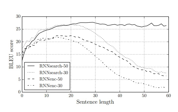Fig 5: BLEU scores for sequence lengths [8]

The BLEU score is simply a metric that compares how good an output text from the model is close to the true reference text. It does so by matching N-grams and the higher the score the better. You can read more on this on machinelearningmastery

Also, in this architecture, the context vector ( h₈) is the same for every time step. Say the network got the first output wrong.. then the entire error kind of propagates forward and since the context is the same at each step, the network has no way to correct itself easily [10].

Building towards Attention

We have spent a lot of time understanding how encoder-decoder models work! The need for understanding encoder-decoder models is because attention was first introduced [9] to solve the main limitation of this architecture and understanding this will help us get an intuitive sense of how it solves the problem.

So far we have established that our main limitation is that a single static context vector is not enough to efficiently encode all input information of long sequences.

Well, the logical solution is to simply have multiple context vectors that change at each time step and feed them into the decoder at each time step.

Also, remember that in the sequence to sequence architecture (refer to Animation 2), in the encoding process we had only used the last hidden state of the encoder h₈ in the decoding stage and discarded all previous hidden states.

The encoder computes hidden states h₁, h₂, ..., h₈. Instead of discarding all this information we can use these hidden states for the decoding process - remember again that we can loosely assume that these are features extracted from the input vectors. Also, the purpose of the context vector is to somehow give us information on the input context. Thus the context vector that will be passed to the decoder at time step t should be influenced by:

1. The previous hidden state of the decoder
2. The hidden states of the encoder h₁, h₂, ..., h₈ - these are information about the input features

Again, if we think logically, consider we are generating the output at time step 2 i.e. op₂. Each of the input hidden states (extracted features from each input word) is not really equally important for generating op₂. Some of the features might be more/less important than the others. Depending on the output we are generating, we need to assign a certain weight (attention) to each of the input features.

The weight that we assign to each input feature depending on the output we have generated so far is called attention

Here we have simply assigned weights to each hidden state/input feature. Note how equation 2 simply looks like a weighted average, where we assign different weights to the different input features at each time step based on the outputs generated (s_t-1 encodes information of the previous outputs generated). Equation 2 simply tries to compute a context vector at each time step based on how important each of the input features is necessary for predicting the word that comes after the hidden state s_t-1.

The next question is how to come up with these weights for each input feature at each time step? The authors of the original attention paper [9] initially proposed to use a feed-forward neural network to figure this out. So this net receives an input feature vector and the previous hidden state vector and comes up with a scalar weight which is the attention weight to assign to that feature at that time step.

In this way, we calculate a set of attention weights for each time step t. Again, to normalize these weights and interpret them as probabilities, we pass these weights through a SoftMax operation.

Note that since we are considering the previous hidden state s_t-1 while calculating each weight itself, we can simplify equation 2 as :

As mentioned before, this is a weighted average over the input features where the weights are learned based on the i/p feature and the output generated so far. Thus we have solved the problem of the context vector being a single static vector which was not enough to summarize the input features efficiently, we now have a mechanism to compute the context vector dynamically at each time step.

We have understood the math behind the attention mechanism and hopefully, you can now appreciate the intuition behind it. In the animation below I have attempted to visualize the entire process. Assume we start right after the Encoder has finished training and given use the set of input features/hidden state vectors [h_1, h_2, ... h_8].

Animation 5 - Full Attention mechanism process

1. h₁, h₂, ..., h₈ are the outputs of the encoding process
2. At each time step we compute a set of attention weights using the function f_att which takes as inputs:
   1. The hidden state of the decoder
   2. The input hidden state we are computing the attention weight for
3. Using the set of attention weights we compute a weighted average w.r.t the input features to get the context vector for that time step
4. The Decoder takes as inputs:
   1. The context vector we just computed
   2. The previous hidden state
   3. The previous output embedding
5. The decoder outputs a new hidden state which gets mapped to an output token and the entire process repeats

Note that in the animation I have not shown the normalization process for the attention scores for sake of simplicity.

Another thing worthwhile to note is that the main output of the attention mechanism is the context vector c_t which is fed to the decoder at every time step. The decoder network is exactly the same as before. You can choose any architecture for the decoder as long as it can take in the context vector at each time step. So from the next part, we will only focus on the output of the attention mechanism and not particularly on the decoder part as that part can change based on what task we are solving for.

---

Next steps

Part 2

We have understood how attention works and why it is needed. We have used a neural network to learn the function f_att, which is a perfectly reasonable approach but we will see in the next post how we can simplify and generalize this. Also note that we have abstracted the process so that [h_1, h_2, ..., h_8] are in no way constrained to be outputs of an RNN or even textual features - they are simply input features. However, we are expected to provide a sequence of vectors s₀ -> s₁ -> ... -> s₇, one by one and get the attention weights for that time step. So we can't quite parallelize this process yet - we will see how we can re-frame the architecture to optimize for this in the next post.

In the next post, we will work our way through a set of abstractions at the end of which you can simply imagine attention as a mechanism to simply throw in whenever you have some input features and want to generate outputs in a sequence.

---

Cite this article as:

@article{sen2021attention,
  title   = "Attention mechanism - An In-depth Analysis and Walkthrough - Part 1",
  author  = "Sen, Shaunak",
  journal = "https://shaunaksen.hashnode.dev",
  year    = "2021",
  url     = "https://shaunaksen.hashnode.dev/attention-mechanism-an-in-depth-analysis-and-walkthrough-part-1"
}

If you have any queries, spotted any errors, or simply want to leave feedback, do contact me at shaunak1105@gmail.com.

---

References

[1] Vaswani, Ashish, et al. “Attention Is All You Need.” ArXiv.Org, 12 June 2017, https://arxiv.org/abs/1706.03762.

[2] Sutskever, Ilya, et al. “Sequence to Sequence Learning with Neural Networks.” ArXiv.Org, 10 Sept. 2014, arxiv.org/abs/1409.3215.

[3] Mikolov, Tomas, et al. “Efficient Estimation of Word Representations in Vector Space.” ArXiv.Org, 7 Sept. 2013, arxiv.org/abs/1301.3781.

[4] Olah, Christopher. “Deep Learning, NLP, and Representations - Colah’s Blog.” Home - Colah’s Blog, 7 July 2014, colah.github.io/posts/2014-07-NLP-RNNs-Repr...

[5] Bloem, Peter. “Machine Learning @ VU | MLVU.” MLVU, mlvu.github.io. Accessed 22 Aug. 2021.

[6] Brownlee, Jason. “Softmax Activation Function with Python.” Machine Learning Mastery, 18 Oct. 2020, machinelearningmastery.com/softmax-activati...

[7] Weiss, Ron J., et al. “Sequence-to-Sequence Models Can Directly Translate Foreign Speech – Google Research.” Google Research, 2017, research.google/pubs/pub46151.

[8] Cho, Kyunghyun. “Introduction to Neural Machine Translation with GPUs (Part 2) | NVIDIA Developer Blog.” NVIDIA Developer Blog, 15 June 2015, developer.nvidia.com/blog/introduction-neur...

[9] Bahdanau, Dzmitry, et al. “Neural Machine Translation by Jointly Learning to Align and Translate.” ArXiv.Org, 1 Sept. 2014, arxiv.org/abs/1409.0473.

[10] Weng, Lilian. “Attention? Attention!” Lilianweng.Github.Io/Lil-Log, 2018, lilianweng.github.io/lil-log/2018/06/24/att...